Data Sources
The estimations reported for every day correspond to the model estimations using information available up to each corresponding day.
Technical Information
Overview of this tool
The tool is based on a statistical model that measures the degree of fluctuation in commodity prices in futures markets. Specifically, it estimates the returns to commodity trading in those markets as reflected in day-to-day percentage changes of futures market prices closest to maturity. When the number of days with extreme positive price changes is high compared to what is expected by the model, the tool alerts that we are in a period of high price volatility.
The first graph above identifies abnormalities or excessive price variability – price volatility that exceeds a pre-established threshold. The red vertical lines on the first graph indicate when daily price increases are very high compared to past returns. This first graph can be compared to the price trend of the commodity, shown in the second graph above.
What the tool identifies
Periods of excessive price variability. This occurs when we observe a large number of extreme positive returns in the three months preceding the day in question. An extreme positive return is defined as a return that exceeds a certain pre-established threshold. This threshold is normally taken to be a high order (95% or above) conditional quantile, (i.e. a value of return that is exceeded with low probability: 5% or less).
Days that are within periods of (high, moderate or low) price variability. This reflects the number of days in the current level of variability based on the number of extreme daily price increases seen over the last three months. For example, 20 days of low variability means that in each of the last 20 reported days, the number of days in the preceding three months with extreme daily price increases was within normal levels.
How the model works
The model works in two steps. First, the threshold to identify extreme positive price returns is calculated based on the 95th percentile of the last 4000 observations. The tool uses the ‘conditional value at risk’ (CVaR) of returns as the threshold, which is a standard measure of risk in financial economics. When a daily return is higher than that threshold, it counts as one day where there was an unusual high price return.
The second step of the model involves counting the number of days in the past three months that experienced such a high daily price increase. When this total number is higher than what is expected by the model, a period of high price variability is indicated. Specifically, the probability that we will observe k days of extreme price returns (returns above the 95% quantile as explained in the definition of excessive price variability) in a period of D consecutive days is defined as:
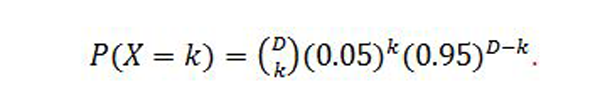
We implement a one-sided test based on a normal approximation for the binomial distribution, using a period of 60 consecutive days that precede any date (i.e. D=60).
The decision rule embedded in the color system
- RED or Excessive Volatility: If the probability value is less than or equal to 2.5%, the null that violations (i.e. days of extreme price returns) are consistent with expected violations is highly questionable, meaning that we are in a period of an excessive number of days of extreme price returns relative to that expected by the model ; therefore we characterize that date as belonging to a period of excessive volatility.
- ORANGE or Moderate volatility: If the probability value is bigger than 2.5% or less than or equal to 5%, the null that violations are consistent with expectations is questionable at a low level, meaning that we are in a period of moderate number of days of extreme price returns relative to that expected; therefore we characterize that date as belonging to a period of moderate volatility.
- GREEN or Low volatility: If the probability value is bigger than 5%, we accept the null that violations are consistent with expectations, meaning that the number of extreme price returns is consistent to what is expected from the model; therefore we characterize that date as belonging to is a period of low volatility.